Microcontroller-Driven Robotic Arm with Software Integration
For my Matura thesis I designed and built a robot arm from consumer electronics and affordable materials, and programmed it to emulate the positioning capabilities of an industrial robot arm.
The arm is driven by an Arduino UNO and six servo motors and is piloted with joysticks. On the software side I derived two mathematical control methods for positioning the end-effector, implemented them as a C++ library, and ran a series of user tests to compare them.
The hardware
The arm uses six servos with torques matched to their position in the chain: 40 kg/cm at the base and shoulder, 10 kg/cm at the elbow joints and 2.2 kg/cm at the hand. The structure is built from 2 mm plywood sheets, cut and glued in layers with instant glue, which soaks through the fibers and hardens the wood completely. The shoulder link is reinforced with an aluminum skeleton, with plywood layers molded to its shape to keep the weight down.
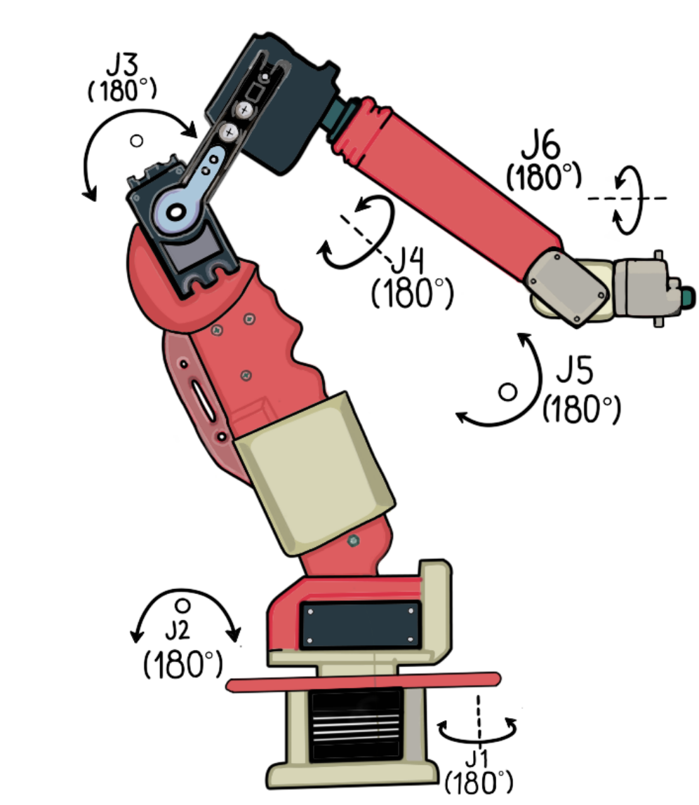
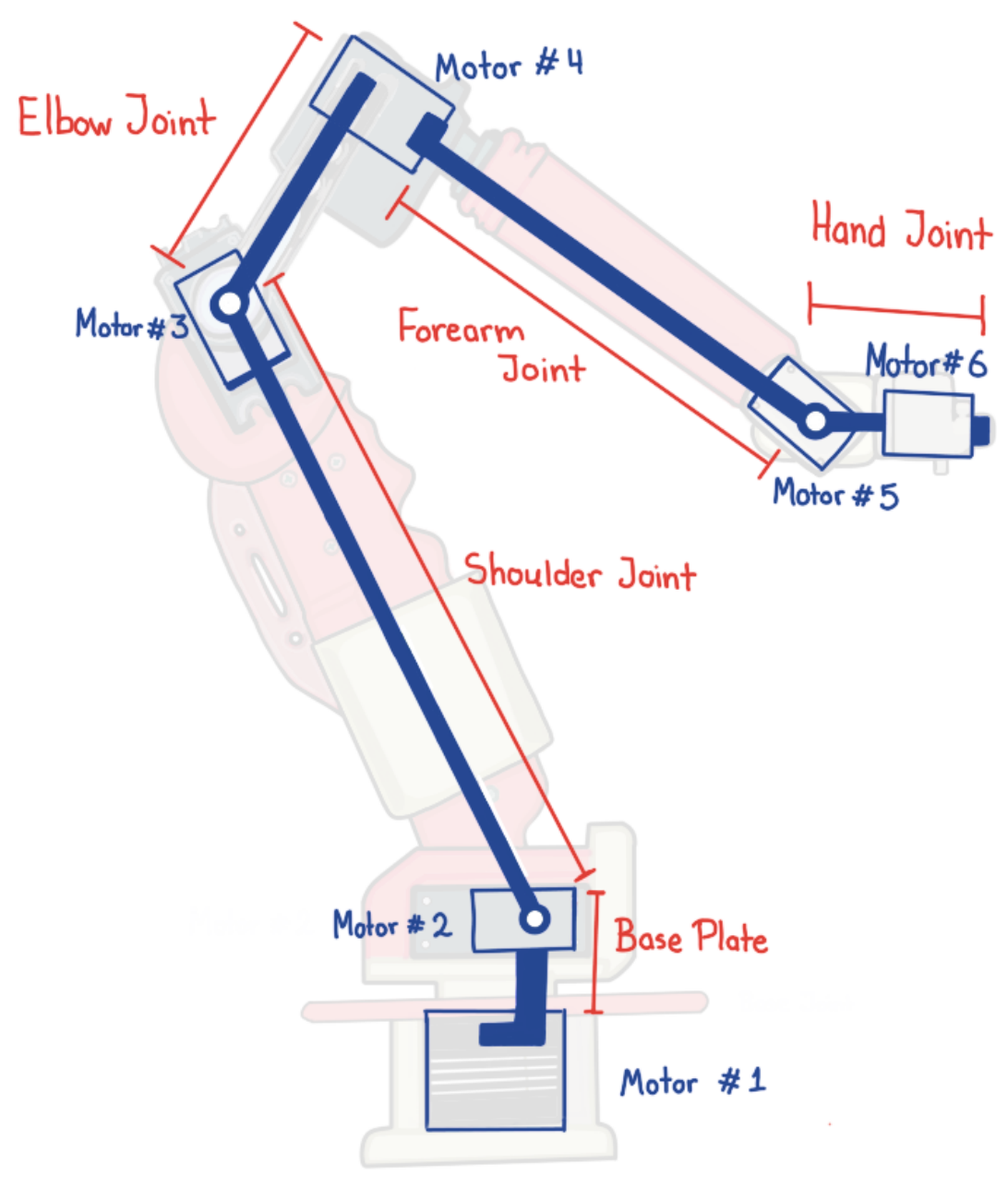
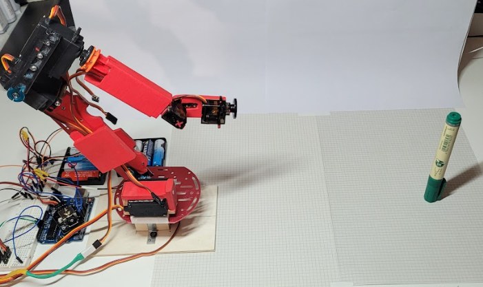
A wide, flat base plate keeps the whole structure from tipping over and houses the strongest servo. The main design decision is at the elbow: the fourth motor is displaced 6.7 cm above the third servo's axis and rotated by 90°. The absolute range of the joint stays the same, but the elbow no longer runs into the shoulder, so the arm can fold completely into itself without colliding with its own structure, and it gains 6.7 cm of forward reach at full stretch.
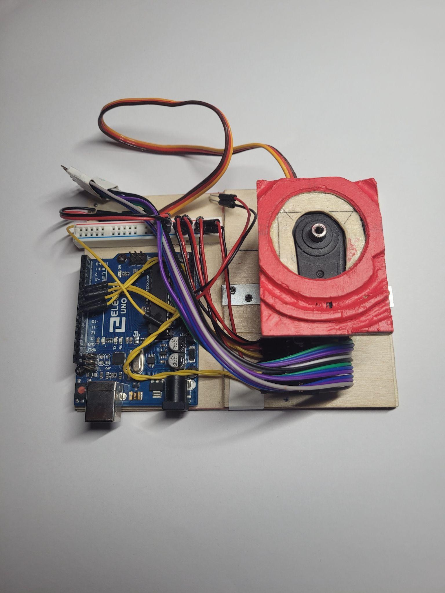
Base plate, upper view, with the Arduino.
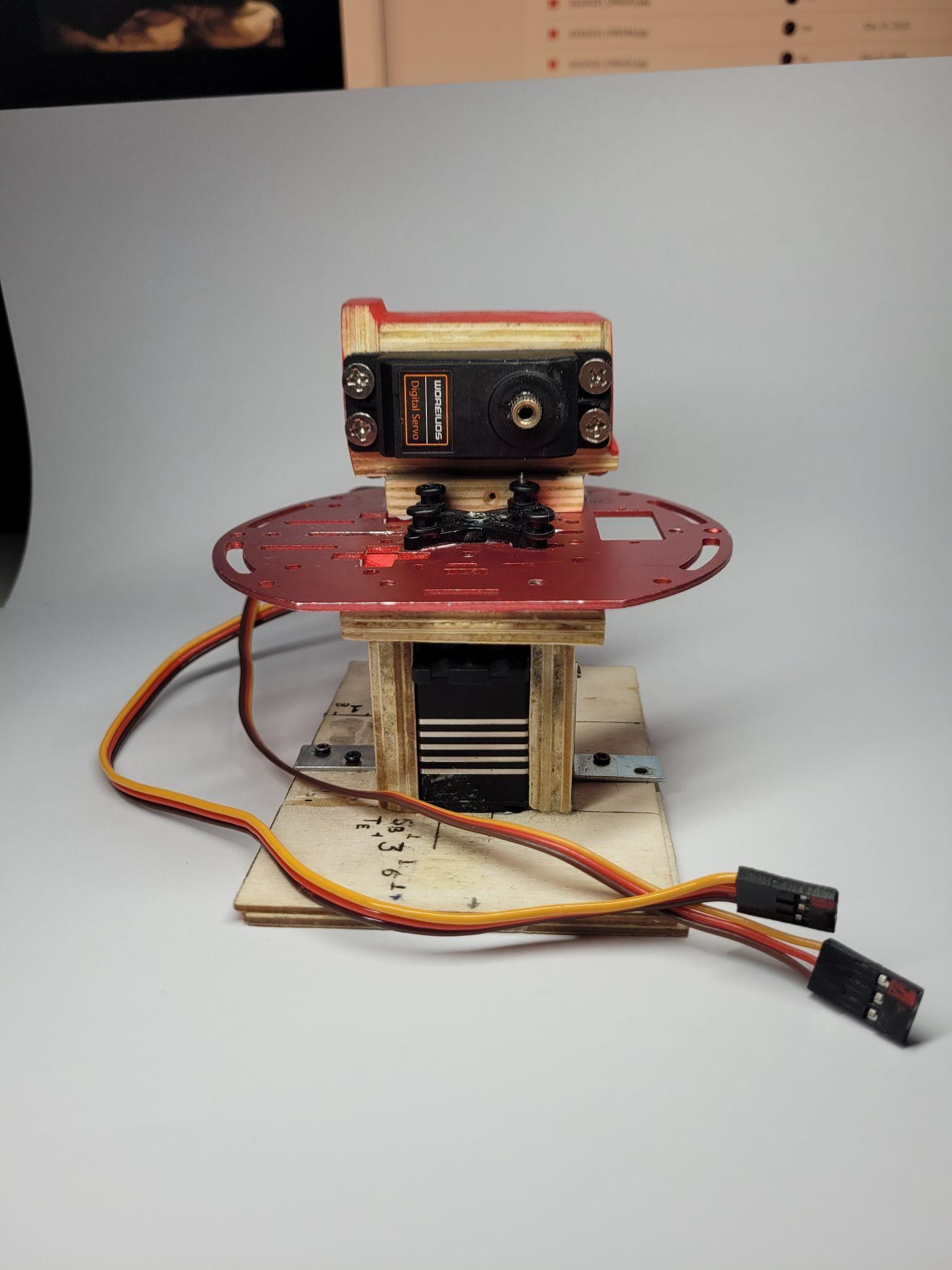
Base plate with the shoulder servo mounted.
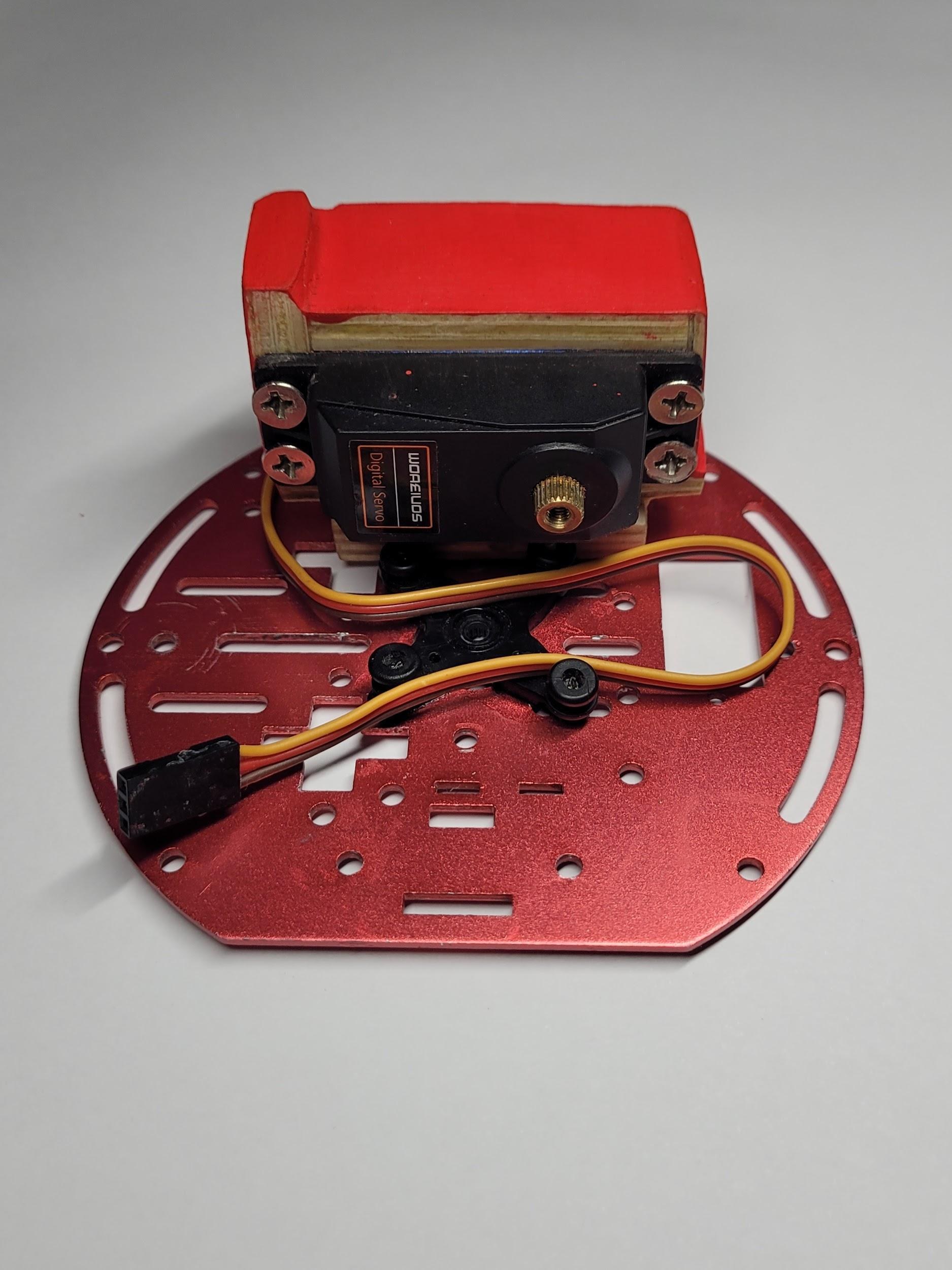
Shoulder servo, front view.
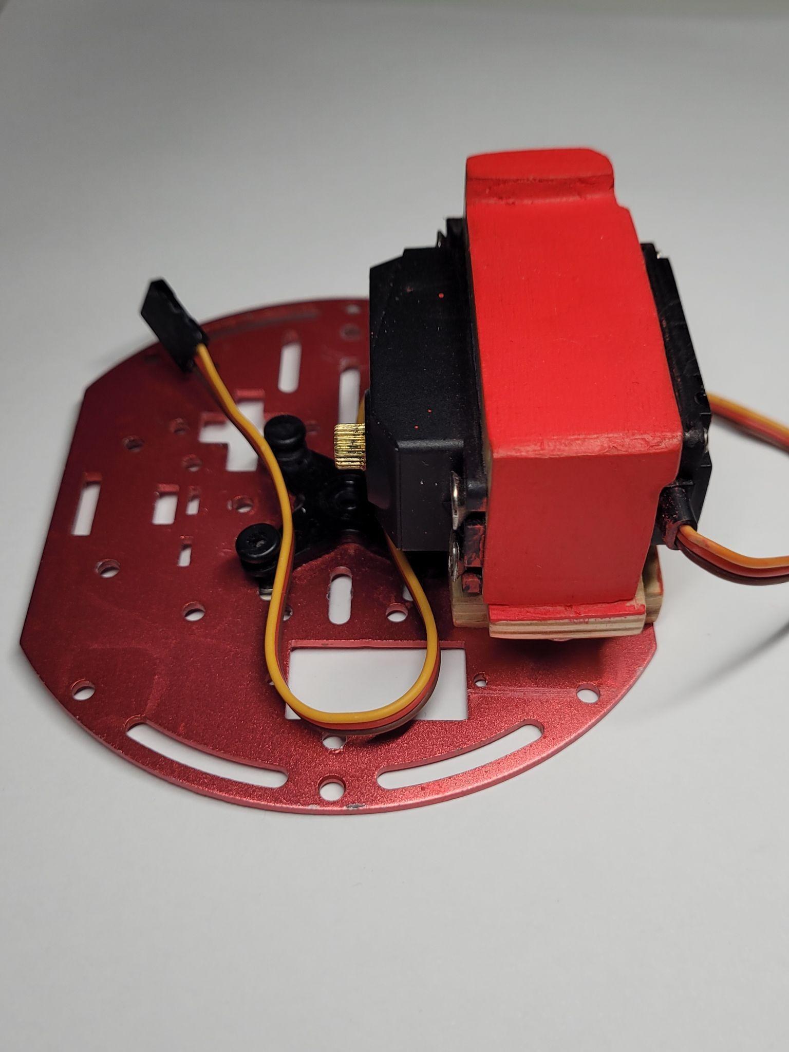
Shoulder servo, side view.
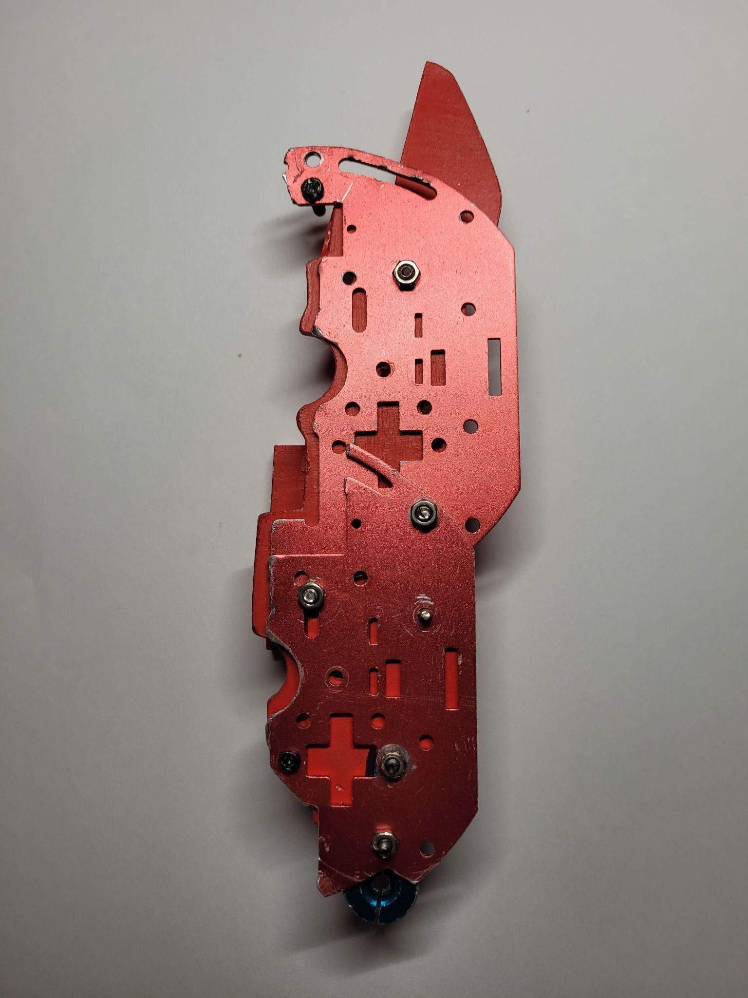
Metal body of the shoulder link.
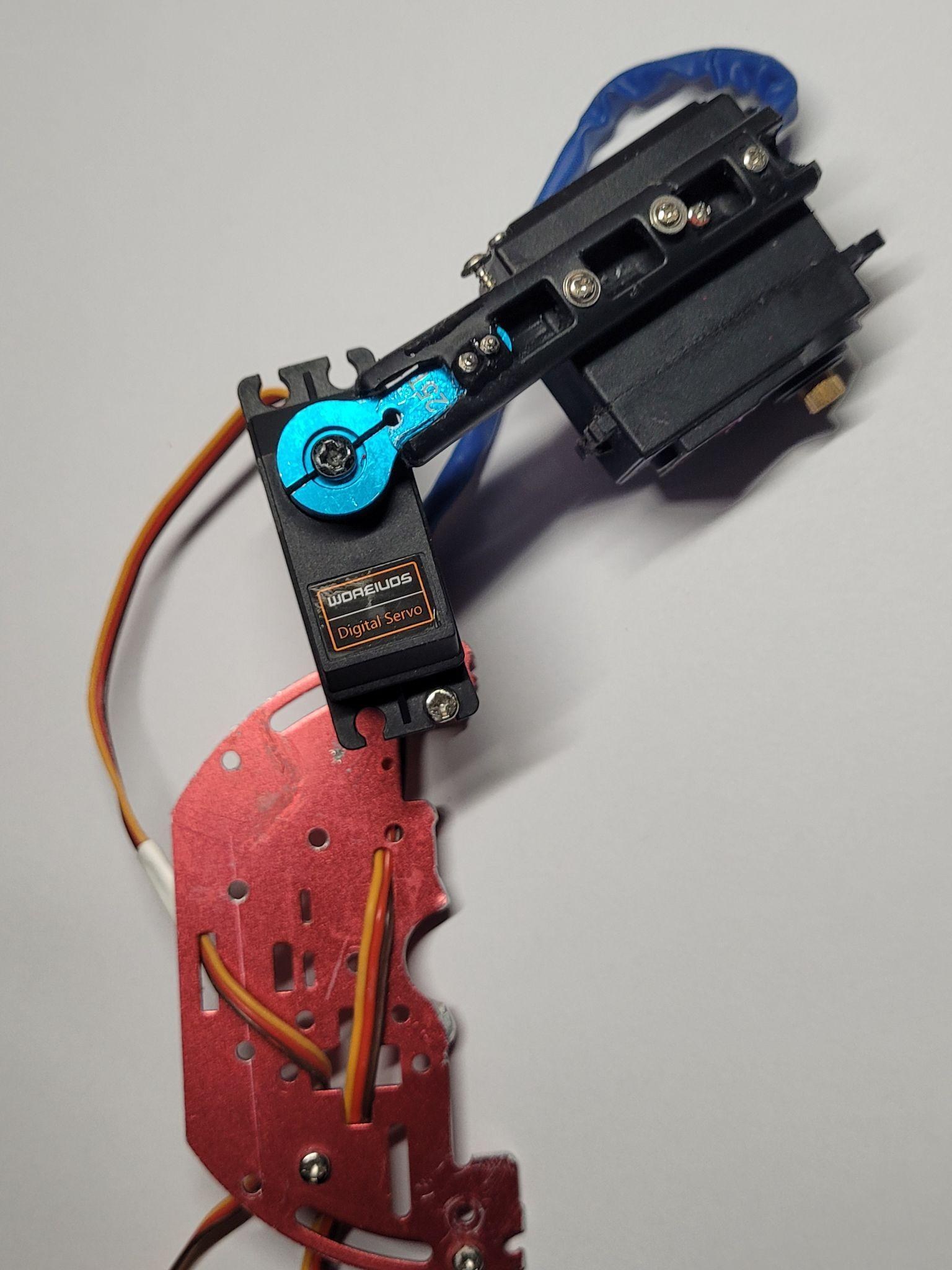
Metal body connected with the elbow servo.
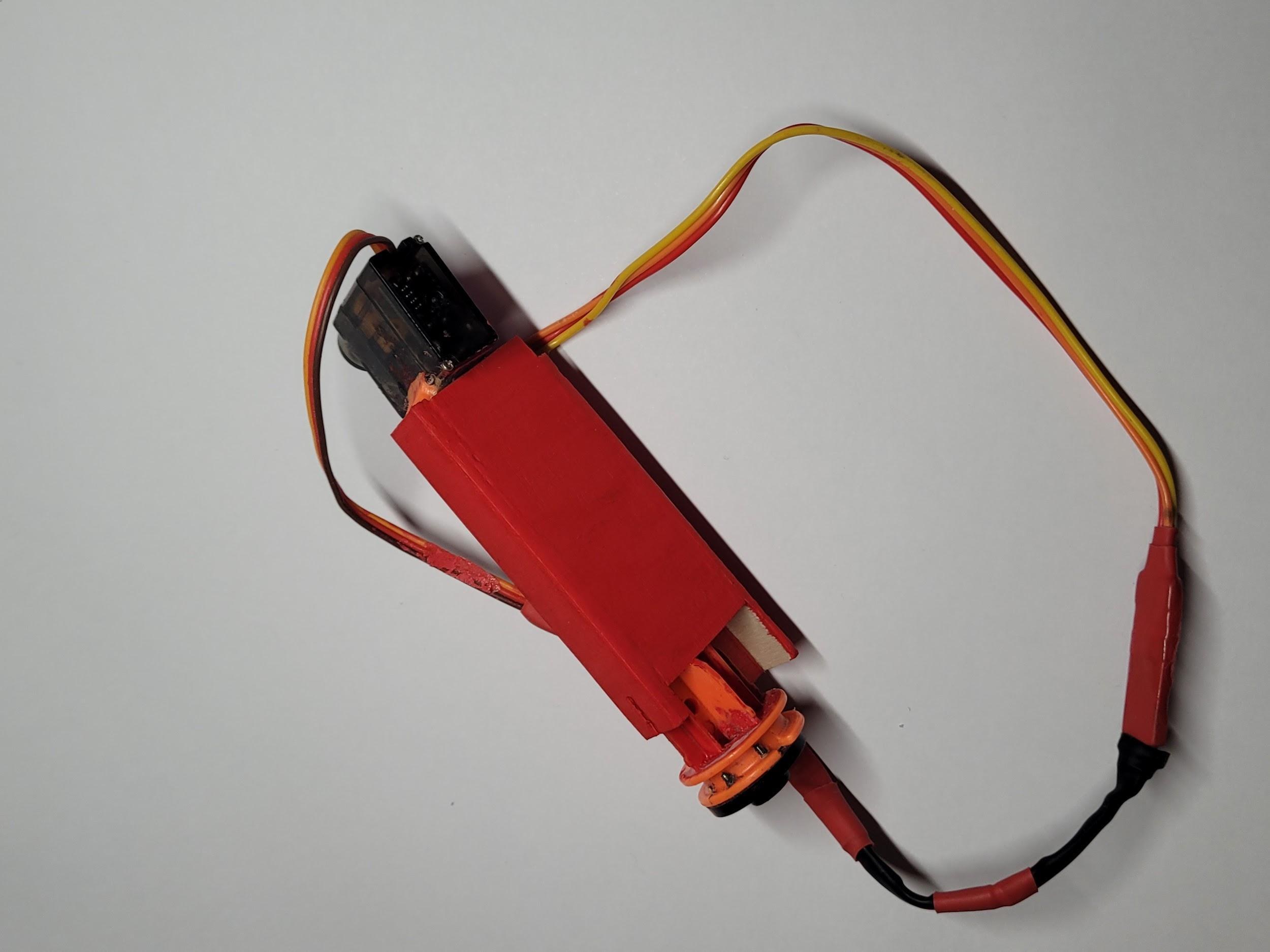
Forearm joint.
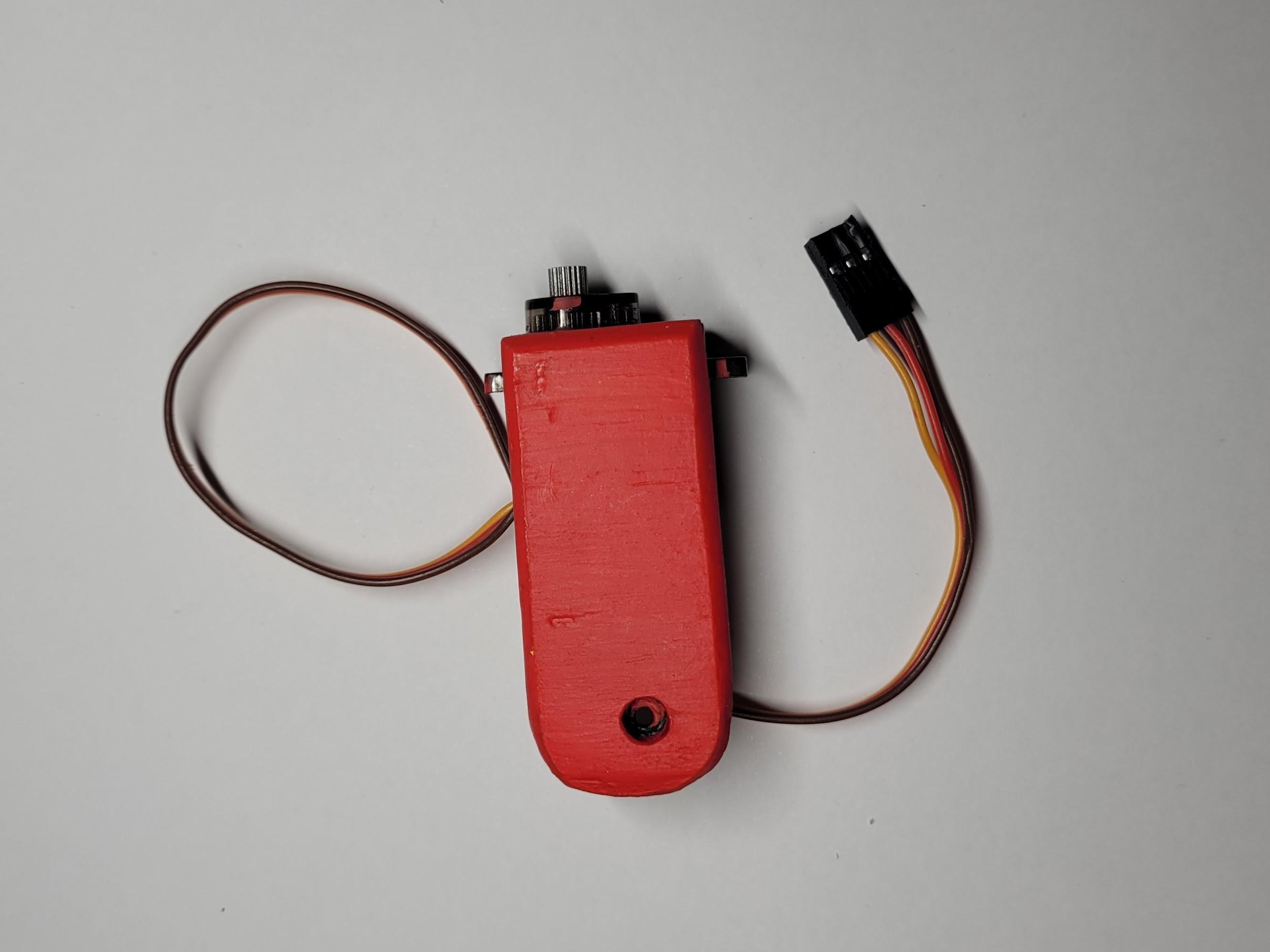
Hand joint.
The base, shoulder and elbow servos draw too much current to run off the Arduino, so they get an external supply: two sets of four AA batteries connected in parallel, 6 volts with double the amps. The three smaller servos run off the Arduino's 5 V pin. Input comes from two joystick modules, a 2-axis one that maps to x and y movement and a 1-axis one for pivoting the hand.
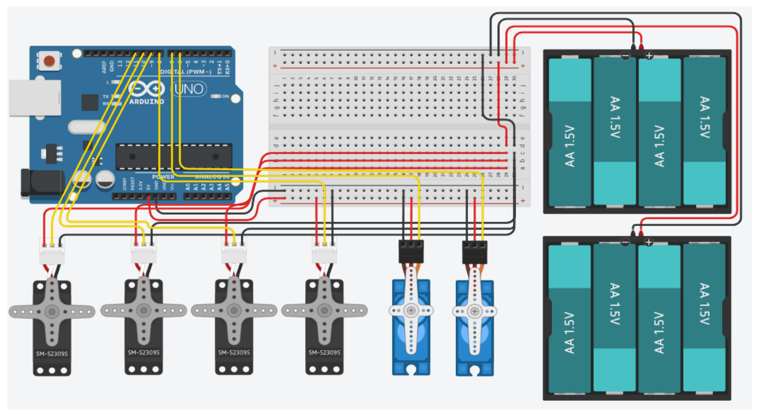
Deriving the kinematics
The control problem is in the vertical plane: the shoulder, elbow and hand joints position the end-effector in 2D. Adding up the horizontal and vertical components of each link with sines and cosines gives the forward kinematic equations, the position of the end-effector as a function of the joint angles.
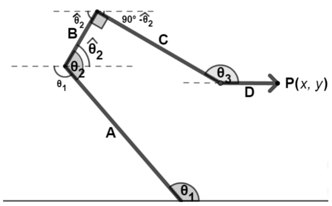
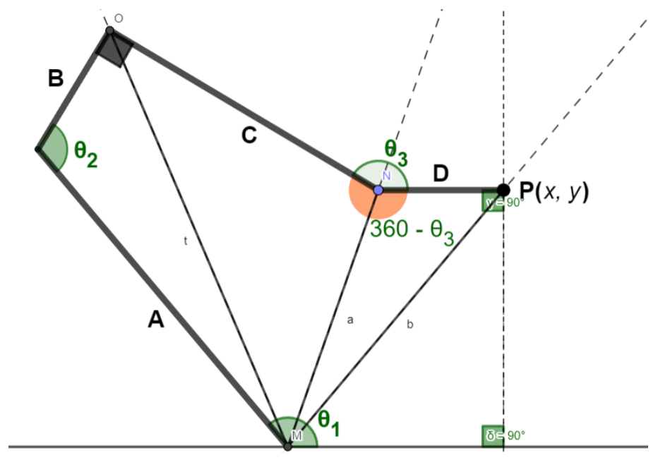
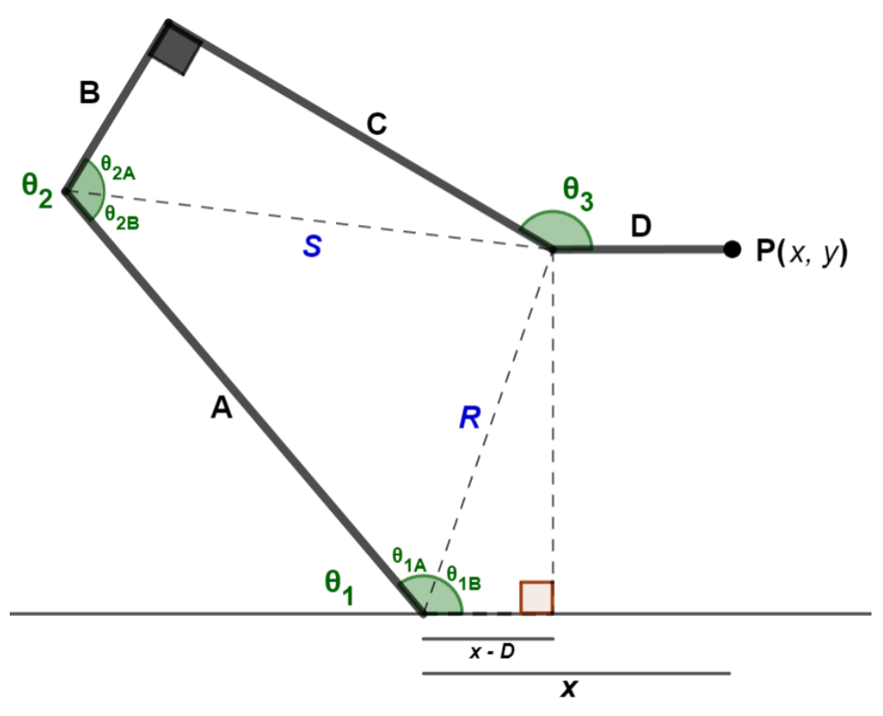
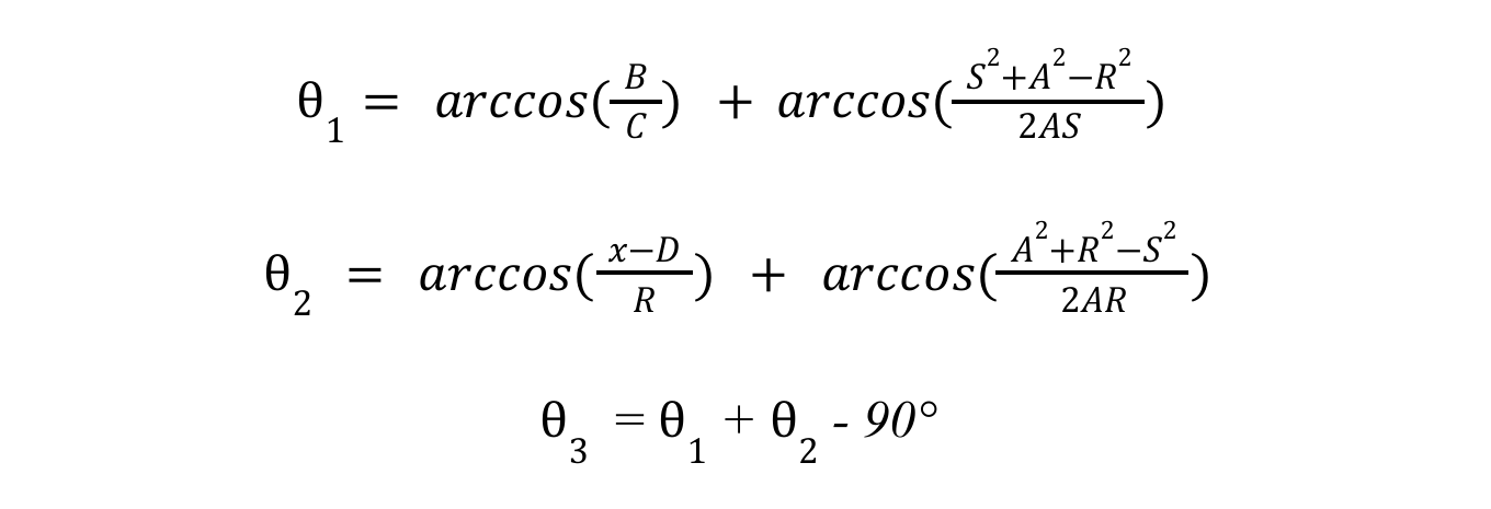
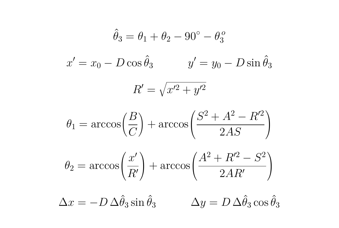
The first method is an exact trigonometric inversion. A 3-jointed system has infinitely many solutions for a given point, so the orientation of the end-effector is fixed parallel to the ground. Drawing a vertical line through the target point closes the arm into a polygon that divides into four triangles, and their internal angles give θ3 in terms of θ1 and θ2, which reduces everything to a two-joint problem. Bisecting the two remaining angles with the segments S and R lets the law of cosines solve the rest.
The second method is an approximate local inversion. Instead of solving for an absolute coordinate, it takes a small displacement (Δx, Δy) and computes the joint angle changes that produce it. The forward kinematic functions are differentiable, so a small change in the angles maps to a small change in position through their Jacobian. As long as that Jacobian is not singular, the inverse function theorem lets me turn the relationship around and solve for the angle changes from the displacement.

The entries of the Jacobian are just the partial derivatives of the forward kinematic functions, which I already had. The problem is singular configurations, where the Jacobian cannot be inverted. In two dimensions the simplest test is its determinant: where it goes to zero the method breaks down, so the software has to keep the arm away from those regions.

Solving the inverted system with Cramer's rule gives a closed form for the angle changes in terms of the displacement.
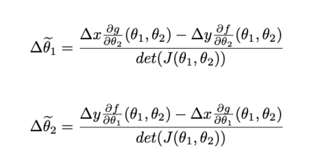
It is less exact than the trigonometric method, but it is more general: the same idea extends to 3D and to arms with more joints, where exact trigonometric solutions stop existing.
Both methods keep the hand parallel to the ground, which means the arm cannot approach objects from the top or the sides. The fix for this is the pivoting solution: rotate the hand joint while moving the wrist to new coordinates that keep the end-effector pinned in place. Both methods got their own version of this correction.
The one-axis joystick only says whether the hand should turn clockwise or counter-clockwise. Calling the hand's angle to the x-axis θ̂₃, the wrist has to move to the point that sits one hand length D behind the end-effector along that angle. Those new coordinates x' and y' go into the trigonometric equations in place of x and y, with the wrist radius R' replacing R. For the derivative method the same rotation becomes a small displacement Δx, Δy of the wrist, which equation 4.4.1 turns into the joint angle changes.
The software
Everything runs as C++ on the Arduino, structured as a small library. A ServoArm class wraps each motor and maps arm angles to servo instructions through a calibration range, since the cheap servos are imprecise and some are mounted mirrored. A Robot class coordinates the joints, exposes methods like moveBy and rotateHandBy, and can switch between the exact and the derivative method at runtime. Every projected move is checked against the servo limits and a stability threshold before it executes, and rejected moves are logged over serial.
The joysticks get their own classes that turn the analog readings into displacement deltas on every cycle of the control loop. The whole library is public on GitHub.
Testing it on people
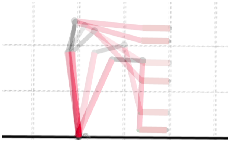
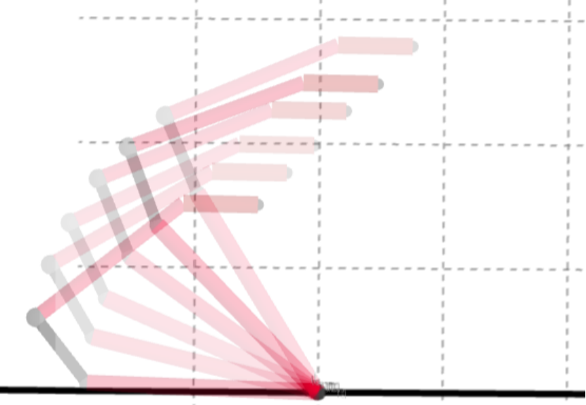
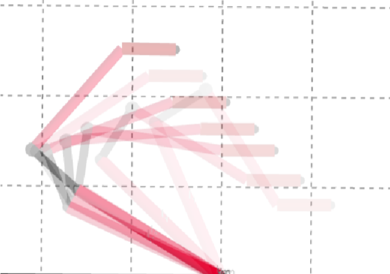
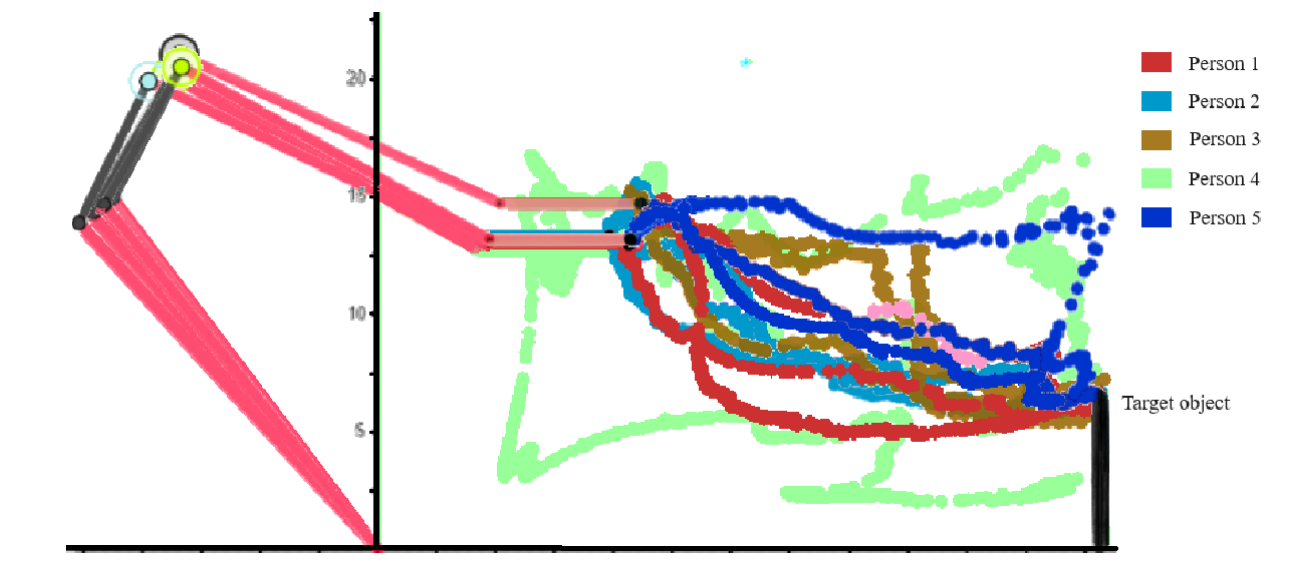
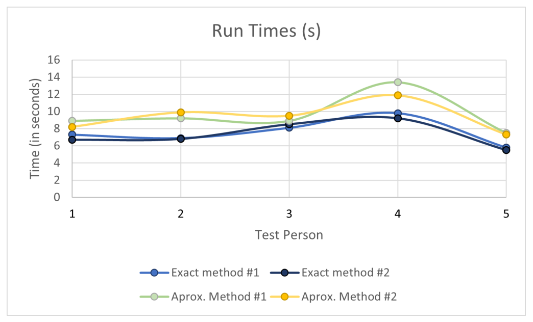
To compare the two methods I ran tests with five participants. In the first protocol they piloted the end-effector along horizontal, vertical and diagonal paths with both methods, then answered yes-or-no questions about correctness, smoothness and input delay. In the second protocol they had to drive the arm to a marker on the table and tip it over within ten seconds, twice per method.
Horizontal path.
Vertical path.
Diagonal path, 45°.
Diagonal path, 135°.
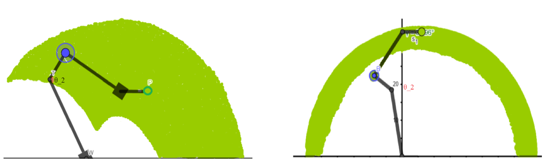
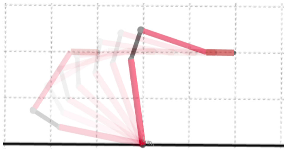
The robot printed its coordinates over serial every 100 ms, so every run could be plotted afterwards in GeoGebra. Of the 20 runs towards the object, 18 succeeded. The exact method took people to the target on straighter paths with fewer corrections, while the derivative method took longer on average, and the only two failed runs were both with it.
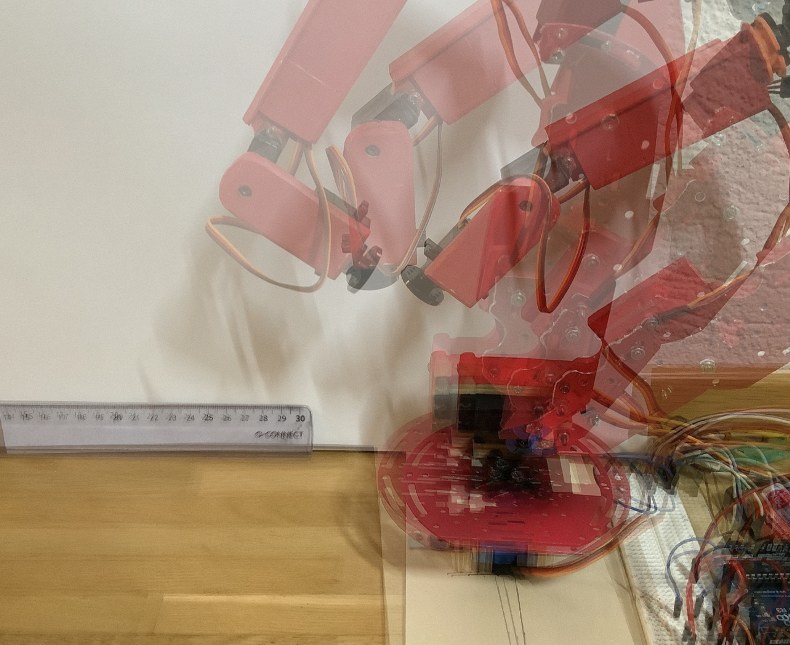
The pivoting test measured how far the end-effector drifts from its position while the hand rotates from 0° to 180° and back. The exact method stayed within 1.5 cm of the starting point. The derivative method accumulated error along the rotation and drifted 4.1 cm, which makes it unusable for pivoting in practice.
The result is a tradeoff: the exact method wins on precision and smoothness but does not extend cleanly to 3D, while the derivative method is approximate but generalizes to higher dimensions and more joints. Most of the remaining error was hardware: cheap potentiometer servos with around 1° of resolution, hand-cut parts and link lengths that are hard to measure precisely. A 3D printer and better actuators would remove most of it.
This post is a condensed version of my Matura thesis, "Microcontroller-Driven Robotic Arm with Software Integration" (MNG Rämibühl, January 2024). The full paper, with the complete derivations, the code walkthrough and all test tables, is available as a PDF: read the full thesis.
The C++ library is on GitHub: github.com/alerest285/robotic_arm.